The Critical Brain Hypothesis

In the spirit of the yearly Society for Neuroscience (SfN) conference, I wanted to clean up and post this review which I have had in the archives for some time. I am publishing this from the Better Buzz coffee shop in San Diego, on the first non-rainy day, and am about to head to the convention center to check out some posters.

The view from my hotel balcony in San Diego (at the Humphreys Half Moon Inn for anyone interested).

This post is a short continuation of the discussion of phase transitions from the previous post. In this post, we review the theory that the brain self-organizes or fine-tunes near the critical point of a second-order phase transition between ordered and disordered states, known as the critical brain hypothesis. We begin by reviewing classical phase transitions, talk about the critical brain hypothesis within this presented framework, and then develop and experimentally study the critical properties of a stochastic branching process that is modeled after recurrent layers of neurons. Finally, we derive the critical exponents of the branching process under a mean-field approximation, and compare them to our in-silico experimental observations and previously published in vivo results.

Introduction

As a quick recap, phase transitions [8] [25] [26] are phenomena first observed in nature, where small changes in a control parameter (temperature, for example) leads to dramatic changes of the quantitative properties or state of an object (the order parameter). Traditionally, the types of phase transitions are categorized into either first-order or second-order phase transitions, called the Ehrenfest Classification [7]. First-order phase transitions undergo a discontinuous change in the order parameter through the phase transition, whereas second-order phase transitions undergo a continuous change. To give a concrete example of this, given the control parameter temperature, and a constant pressure of 1 atm, a liquid will undergo a first-order liquid-to-gas phase transition at the critical temperature of 100 degrees Celsius. This is a first-order transition in the sense that at exactly 100 degrees Celsius there is a discrete change in its properties. Across many dynamical systems that undergo phase transitions, unique properties have been observed near or at critical points including long-range dynamic correlations and scale-free dynamics. For more details, see my previous post.

The critical brain hypothesis [1] [2] [10] [11] [12] [14] [17] [18] [19] [20] [21] proposes that biological neural systems operate at or near the critical point of a second-order phase transition, balanced between ordered and disordered states. One of the reasons it may be advantageous for the brain to either self-organize or fine-tune [2] [9] [15] [16] near criticality is that, from an information-theoretic standpoint, systems at criticality exhibit optimal information transmission, and may even achieve a balance between efficient and generalizable encoding of information [3]. More evidence for criticality in the brain comes from the observation that neuronal avalanches, which are cascades of neural activity that propagate through networks following the characteristic patterns of critical systems, exhibit scale-free dynamics in their relative size and lifetime distributions (which follow power laws). Recent experimental evidence using various recording techniques, from single-neuron measurements to large-scale brain imaging, has revealed signatures of criticality across different scales, including power-law distributions of neural activity, long-range dynamic correlations, and critical fluctuations [1]

There are also three other threads of research in criticality that I find interesting, but will not go too much into. These are: (1) Understanding biologically how the brain could either fine-tune or self-organize near the critical point [13] [15], (2) the clinical relevancy of criticality in the brain [23] [24], and (3) other miscellaneous directions of research that I found interesting [5] [6].

A Stochastic Branching Model

To study and formalize these concepts mathematically, we simulate a stochastic branching process that models the simplified dynamics of activity propagating through layers of neurons. Below is an interactive figure that allows you to simulate the branching process for varying initial conditions and values of the coupling strength $J$ .

You can play with this interactive figure to study supercritical brain dynamics by cranking up the value of the order parameter $J$ , or subcritical brain dynamics by reducing the value of $J$ . The initial sites parameter controls the initial value.

More formally, we consider a network in which individual neurons can activate other neurons through a probabilistic weight matrix. The state of each neuron $i$ at time $t$ is represented by $a_i^{(t)} \in \{0, 1\}$ , indicating whether the neuron is active (1) or inactive (0). Then, let $p_{ij}^{(t)}$ be the conditional probability that neuron $j$ becomes active at time $t+1$ given that neuron $i$ was active at time $t$ . That is

p_{ij}^{(t)} = P(a_j^{(t+1)} = 1 \mid a_i^{(t)} = 1)

Furthermore, these connection probabilities satisfy the normalization condition

\sum_{j=1}^{N} p_{ij}^{(t)} = 1

for all source neurons $i$ and times $t$ . This ensures that the total probability of activation flowing from any source neuron sums to one (see Figure 1 for intuition).

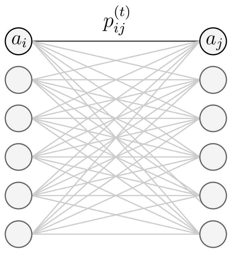
**Figure 1:** A small illustration of the stochastic branching model. The model is a simple network of neurons that can activate other neurons in subsequent layers through some probability of activation.

Given this framework, we define the update rule for activity propagation as

a_j^{(t+1)} = H\left(J \sum_{i=1}^{N} a_i^{(t)} p_{ij}^{(t)} - r_j\right)

where $H$ is the Heaviside step function, $J$ is the coupling strength (control parameter), and $r_j$ are independent random variables uniformly distributed on $[0, 1]$ for each neuron $j$ at each timestep.

Expected Value Analysis

In analyzing this branching process, we are particularly interested in the conditions under which information transmission is optimized. The key insight is that information transmission in our model is maximized when the output activity statistically preserves the input activity. That is, when $E[a^{(t)}] = a^{(t-1)}$ , where $a^{(t)} = \sum_i a_i^{(t)}$ denotes the total activity at time $t$ . This condition represents a critical balance where the network neither amplifies nor absorbs its input signals (on average), allowing for optimal propagation of information through the system.

Relating this back to our coupling strength $J$ , if $J$ is too low then signals will die out and information will be lost. Else, if $J$ is too high, the system will saturate, lose its ability to discriminate between different inputs, and enter an epileptic-like state. Thus, by examining the expected behavior of our system, we can identify the critical point where information transmission is optimized.

Taking the expected value over the random variables $r_j \sim U(0, 1)$ independently gives

\begin{align*} E[a_j^{(t+1)}] &= P\left(J \sum_{i=1}^N a_i^{(t)} p_{ij}^{(t)} > r_j\right) \\ &= 1 - P\left(r_j > J \sum_{i=1}^N a_i^{(t)} p_{ij}^{(t)}\right) \\ &= \min\left(J \sum_{i=1}^N a_i^{(t)} p_{ij}^{(t)}, 1\right) \end{align*}

Note that because $r_j$ are independent across neurons, we can compute expectations for each neuron separately, which preserves the mean-field dynamics.

To derive the network-level dynamics, we sum over all target neurons $j$

\begin{align*} E[a^{(t+1)}] &= \sum_{j=1}^N E[a_j^{(t+1)}] \\ &= \sum_{j=1}^N \min\left(J \sum_{i=1}^N a_i^{(t)} p_{ij}^{(t)}, 1\right) \end{align*}

Assuming the $\min$ function does not saturate (valid when activity is sparse)

\begin{align*} E[a^{(t+1)}] &= J \sum_{j=1}^N \sum_{i=1}^N a_i^{(t)} p_{ij}^{(t)} \\ &= J \sum_{i=1}^N a_i^{(t)} \left(\sum_{j=1}^N p_{ij}^{(t)}\right) \\ &= J \sum_{i=1}^N a_i^{(t)} \\ &= J \, a^{(t)} \end{align*}

where we used the normalization condition $\sum_{j=1}^N p_{ij}^{(t)} = 1$ .

The relationship $E[a^{(t+1)}] = J a^{(t)}$ reveals how information propagates through the network. At $J = 1$ , we have $E[a^{(t+1)}] = a^{(t)}$ , indicating that the expected activity at the next timestep perfectly matches the current activity. This represents a critical point where

$J < 1$ : Leads to information decay as activity gets absorbed by the network since $E[a^{(t+1)}] < a^{(t)}$ . In this case, activity decays exponentially as $J^t$ .
$J = 1$ : The critical point where information is maximally preserved as $t$ increases. In this case, the expected activity in the next layer matches the current activity $E[a^{(t+1)}] = a^{(t)}$ , and optimal information transmission occurs.
$J > 1$ : Leads to information saturation where activity amplifies until reaching a stable state of saturation where all neurons are active. In a similar way to case when $J < 1$ , the system loses information about the initial conditions as time progresses.

This critical point at $J = 1$ represents a unique balance where the network can maintain and transmit information without loss (on average), making it optimal for the transmission and processing of information. Another way of saying this is that at $J=1$ we are at the optimal point in which observing the activity at some time $t$ for $t>0$ maximally resolves our uncertainty about the initial condition $a^{(0)}$ . Hopefully I have explained this idea in enough ways to at least give some base-level intuition for why criticality might be advantageous for the brain.

Monte-Carlo Simulations

Now that we have mathematically formulated our model, we run a Monte-Carlo simulation to experimentally derive the phase-transition diagrams, compute the dynamic correlation length for varying values of $J$ , and study potential scale-free behavior at $J=1$ .

First, to study the phase-transitions of our model we simulate 10,000 realizations of neural activity on a 20x25 grid (neurons by time) using an initial condition of $a^{(0)}=10$ , and then computed the state of the model as the mean activity in the final layer (Figure 2). Doing so revealed an absorbing state for $J < 1$ , where dynamics quickly get absorbed leading to zero activity in the final layer, and a saturating state for $J>1$ , where the activity quickly saturates all neurons in the final layer. As predicted by our theoretical results, a 2nd-order phase transition occurs at the critical value of $J=1$ where dynamics are optimally maintained without saturating or getting absorbed on average.

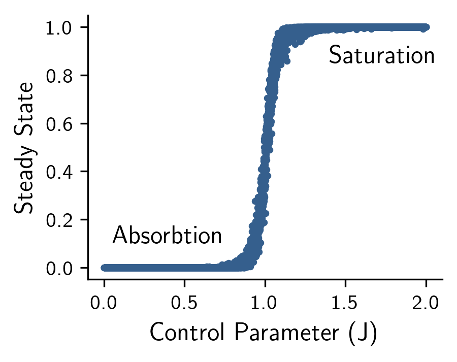
**Figure 2:** The state of the model (y-axis) given varying values of the control parameter J (x-axis). Notice that a 2nd-order phase transition occurs at the critical value of J=1 where dynamics are optimally maintained without saturating or getting absorbed on average.

To study the long-range dynamic correlation, we again simulate a 20x25 grid using an initial condition of $a^{(0)}=10$ across 10,000 realizations, and then used the following equation to measure the correlation of activity at time t from the initial condition as

a^{(0)} - \sqrt{\frac{1}{T} \sum_{t=1}^{T} (a^{(t)} - a^{(0)})^2}

This allows us to study how similar the activations are in layer $t$ from the initial conditions. If the activations $a^{(t)}$ are very different from $a^{(0)}$ then our correlation function should be much less than $a^{(0)}$ . Inversely, for $a^{(t)}$ close to $a^{(0)}$ the correlation function should approach $a^{(0)}=10$ for our experiment. As per our previous mathematical derivation, we would expect the maximum correlation value of $a^{(0)}=10$ to occur at the critical value $J=1$ . Running this experiment (Figure 3) empirically confirms this finding. One can see that at the critical value $J=1$ that $a^{(0)} \approx a^{(t)}$ .

**Figure 3:** The long-range dynamic correlation length (y-axis) given varying values of the control parameter J (x-axis). Notice that the correlation length is maximized at the critical value of J=1 representing critical dynamics.

Finally, inspired by John Beggs initial work on neuronal avalanches [1] [18], we study the scale-free properties of neuronal avalanches near the critical point. To do this, we simulate a grid of size 40x50 at the critical value $J=1$ , and set the initial condition to be $a^{(0)}=1$ . Then, we record the length that the information propagated (the length of the avalanche), and plotted its log-log distribution (Figure 4). If the dynamics are critical, we should expect to see a power-law distribution in the length of the avalanches. During implementation, there is the edge case of when the activity reaches the last layer (layer 50). In this case, we cannot determine the total length of the avalanche as the activity is not yet fully propagated. To handle this, we ablate out any cases in which the activity reaches the last layer (can be seen as clipping the distribution at the last layer). Furthermore, we can set up 2 controls with subcritical and supercritical dynamics, which in theory should not display scale-free behavior. The results can be seen below in Figure 4.

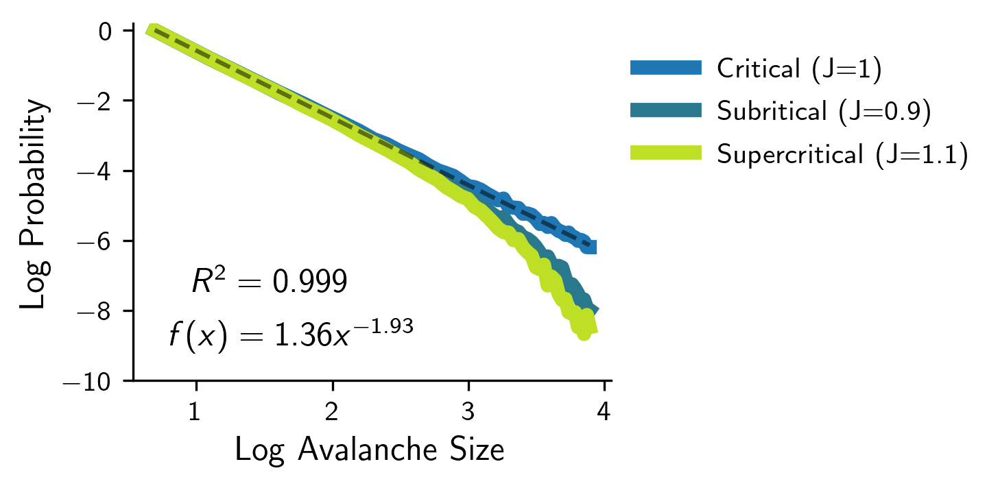
**Figure 4:** The log-log distribution of the length of the avalanches given three different values of the control parameter J at subcritical, critical, and supercritical dynamics. Notice that when J=1, we see a clear power-law distribution (linear line in log-log plot), and when J≠1, we see non-scale-free behavior (curved line in log-log plot).

Doing so revealed a clear power-law when $J=1$ , and non-scale-free behavior when $J \neq 1$ . Furthermore, we computed the critical exponent when $J=1$ to be $\beta=1.92$ . You can look at the Marshall et al. paper [4] for a similar empirical study on simulated models.

Mean-Field Analysis

While the simulations revealed power-law behavior in the lifetime duration of avalanches with exponent $\beta \approx 1.92$ , we can derive this analytically using a mean-field approximation of our branching process. In the mean-field limit, our branching model reduces to the classical Galton-Watson process, where each active neuron independently generates offspring according to a Poisson distribution with mean $J$ .

Let $n^{(t)}$ denote the number of active neurons at time $t$ . The dynamics are then

n^{(t+1)} \mid n^{(t)} \sim \text{Poisson}(J n^{(t)})

An avalanche beginning from $n^{(0)} = 1$ continues until extinction, with length $L$ that we define as the first time $t$ such that $n^{(t)} = 0$ . Formally, this is

L = \min \{ t \geq 1 : n^{(t)} = 0 \}

For critical branching processes where the mean offspring equals 1, we know from early results in probability theory that the survival probability is

P(n^{(t)} > 0 \mid n^{(0)} = 1) \sim \frac{2}{\sigma^2 t}

as $t \to \infty$ , and where $\sigma^2$ is the variance of the offspring distribution. See proposition 5 in section 1.4 of the U-Chicago notes on the Galton-Watson process for a full proof [22]. For $\text{Poisson}(J=1)$ , we have $\sigma^2 = 1$ , yielding

P(n^{(t)} > 0 \mid n^{(0)} = 1) \sim \frac{2}{t}

The avalanche length distribution is then given by

\begin{align*} P(L = t \mid n^{(0)} = 1) &= P(n^{(t-1)} > 0, n^{(t)} = 0 \mid n^{(0)} = 1) \\ &= P(n^{(t-1)} > 0 \mid n^{(0)} = 1) - P(n^{(t)} > 0 | n^{(0)} = 1) \\ &\sim \frac{2}{t-1} - \frac{2}{t} \\ &= \frac{2}{t(t-1)} \\ &\sim \frac{2}{t^2} \end{align*}

Therefore, at criticality the avalanche-duration distribution follows a power law with critical exponent $\beta = 2$ , which is consistent with the mean-field limit of the directed percolation universality class. Our numerical result of $\beta = 1.92$ agrees reasonably well with this result (with finite-size effects on the 2D grid likely contributing for the small deviations). Experimentally, Beggs and Plenz [1] found critical exponents for the duration distribution of avalanches around $\alpha \approx 2.0$ in rat cortical slices. The critical exponent for the avalanche size distribution can likewise be derived, and can be shown for mean-field directed percolation to be $\tau_{MF} = 3/2$ , again matching experimental observations of $\tau \approx 1.5$ in neural systems [1].

For $J \neq 1$ , the power-law behavior we observed at criticality breaks down, as we saw in Figure 4. In the subcritical regime ( $J < 1$ ), recall that activity decays exponentially and signals die out as $J^t$ . This exponential decay of the survival probability translates directly into an exponential distribution of avalanche lifetimes rather than a power-law, since the network is too absorptive to sustain the long-range cascades of neural activity characteristic of critical dynamics. In the supercritical regime ( $J > 1$ ), the situation is reversed, where the network is so excitable that avalanches can have infinite lifetime with positive probability. Mathematically, the extinction probability satisfies $q = P(L < \infty) < 1$ , meaning some avalanches never terminate. This concentration of probability mass at infinity fundamentally prevents power-law behavior. Instead of scale-free dynamics, the network saturates too quickly and loses its ability to discriminate between different cascade sizes. Thus, power-law avalanche statistics uniquely emerge at the critical point $J = 1$ , where the network balances between absorbing and saturating dynamics. This is exactly the regime where, as we showed earlier, information transmission is optimized. For references on this, again see the U-Chicago notes on the Galton-Watson process [22]

[{"id":1,"title":"Neuronal Avalanches in Neocortical Circuits","authors":["Beggs, J.","Plenz, D."],"year":2003,"url":"https://www.jneurosci.org/content/23/35/11167"},{"id":2,"title":"Theoretical foundations of studying criticality in the brain","authors":["Tian, Y.","Tan, Z.","Hou, H.","Li, G.","Cheng, A.","Qiu, Y.","Weng, K.","Chen, C.","Sun, P."],"year":2022,"url":"https://doi.org/10.1162/netn_a_00269"},{"id":3,"title":"High-dimensional geometry of population responses in visual cortex","authors":["Stringer, C.","Pachitariu, M.","Steinmetz, N.","Carandini, M.","Harris, K."],"year":2019,"url":"https://www.nature.com/articles/s41586-019-1346-5"},{"id":4,"title":"Analysis of Power Laws, Shape Collapses, and Neural Complexity: New Techniques and MATLAB Support via the NCC Toolbox","authors":["Marshall, N.","Timme, N.","Bennett, N.","Ripp, M.","Lautzenhiser, E.","Beggs, J."],"year":2016,"url":"https://www.frontiersin.org/journals/physiology/articles/10.3389/fphys.2016.00250/full"},{"id":5,"title":"Behavior of Early Warnings near the Critical Temperature in the Two-Dimensional Ising Model","authors":["Morales, I.","Landa, E.","Angeles, C.","Toledo, J.","Rivera, A.","Temis, J.","Frank, A."],"year":2015,"url":"https://journals.plos.org/plosone/article?id=10.1371/journal.pone.0130751"},{"id":6,"title":"Criticality in Spreading Processes without Timescale Separation and the Critical Brain Hypothesis","authors":["Korchinski, D."],"year":2021,"url":""},{"id":7,"title":"The Ehrenfest Classification of Phase Transitions: Introduction and Evolution","authors":["Jaeger, G."],"year":1998,"url":"https://doi.org/10.1007/s004070050021"},{"id":8,"title":"Phase transitions in biology: from bird flocks to population dynamics","authors":["Heffern, E.","Huelskamp, H.","Bahar, S.","Inglis, R."],"year":2021,"url":"https://royalsocietypublishing.org/doi/10.1098/rspb.2021.1111"},{"id":9,"title":"A devil’s advocate view on ‘self-organized’ brain criticality","authors":["Gros, C."],"year":2021,"url":"https://doi.org/10.1088/2632-072X/abfa0f"},{"id":10,"title":"Being Critical of Criticality in the Brain","authors":["Beggs, J.","Timme, N."],"year":2012,"url":"https://www.frontiersin.org/journals/physiology/articles/10.3389/fphys.2012.00163/full"},{"id":11,"title":"Criticality in the brain: A synthesis of neurobiology, models and cognition","authors":["Cocchi, L.","Gollo, L.","Zalesky, A.","Breakspear, M."],"year":2017,"url":"https://www.sciencedirect.com/science/article/pii/S0301008216301630"},{"id":12,"title":"Is criticality a unified setpoint of brain function?","authors":["Hengen, K.","Shew, W."],"year":2025,"url":"https://www.sciencedirect.com/science/article/pii/S0896627325003915"},{"id":13,"title":"Role of homeostatic plasticity in critical brain dynamics following focal stroke lesions","authors":["Rocha, R.","Zorzi, M.","Corbetta, M."],"year":2024,"url":"https://www.nature.com/articles/s41598-024-80196-6"},{"id":14,"title":"Neuronal Avalanches Imply Maximum Dynamic Range in Cortical Networks at Criticality","authors":["Shew, W.","Yang, H.","Petermann, T.","Roy, R.","Plenz, D."],"year":2009,"url":"https://www.jneurosci.org/content/29/49/15595"},{"id":15,"title":"Cortical Circuit Dynamics Are Homeostatically Tuned to Criticality In Vivo","authors":["Ma, Z.","Turrigiano, G.","Wessel, R.","Hengen, K."],"year":2019,"url":"https://www.cell.com/neuron/abstract/S0896-6273(19)30737-8"},{"id":16,"title":"Self-organized criticality as a fundamental property of neural systems","authors":["Hesse, J.","Gross, T."],"year":2014,"url":"https://www.frontiersin.org/journals/systems-neuroscience/articles/10.3389/fnsys.2014.00166/full"},{"id":17,"title":"Landau–Ginzburg theory of cortex dynamics: Scale-free avalanches emerge at the edge of synchronization","authors":["Santo, S.","Villegas, P.","Burioni, R.","Muñoz, M."],"year":2018,"url":"https://www.pnas.org/doi/full/10.1073/pnas.1712989115"},{"id":18,"title":"Emergent complex neural dynamics","authors":["Chialvo, D."],"year":2010,"url":"http://arxiv.org/abs/1010.2530"},{"id":19,"title":"The criticality hypothesis: how local cortical networks might optimize information processing","authors":["Beggs, J."],"year":2007,"url":"https://royalsocietypublishing.org/doi/10.1098/rsta.2007.2092"},{"id":20,"title":"Optimal Dynamical Range of Excitable Networks at Criticality","authors":["Kinouchi, O.","Copelli, M."],"year":2006,"url":"https://arxiv.org/abs/q-bio/0601037v2"},{"id":21,"title":"Earthquake Cycles and Neural Reverberations: Collective Oscillations in Systems with Pulse-Coupled Threshold Elements","authors":["Herz, A.","Hopfield, J."],"year":1995,"url":"https://link.aps.org/doi/10.1103/PhysRevLett.75.1222"},{"id":22,"title":"Branching Processes","authors":[],"year":"","url":"https://galton.uchicago.edu/~lalley/Courses/312/Branching.pdf"},{"id":23,"title":"Why Brain Criticality Is Clinically Relevant: A Scoping Review","authors":["Zimmern, V."],"year":2020,"url":"https://pmc.ncbi.nlm.nih.gov/articles/PMC7479292/"},{"id":24,"title":"A Shift Toward Supercritical Brain Dynamics Predicts Alzheimer’s Disease Progression","authors":["Javed, E.","Suárez-Méndez, I.","Susi, G.","Román, J.","Palva, J.","Maestú, F.","Palva, S."],"year":2025,"url":"https://www.jneurosci.org/content/45/9/e0688242024"},{"id":25,"title":"Statistical Physics","authors":["Landau, L.","Lifshitz, E."],"year":1980,"url":""},{"id":26,"title":"Statistical Mechanics: An Introductory Graduate Course","authors":["Berlinsky, A.","Harris, A."],"year":2019,"url":""}]

References

Beggs, J., Plenz, D. (2003). Neuronal Avalanches in Neocortical Circuits. Link
Tian, Y., Tan, Z., Hou, H., Li, G., Cheng, A., Qiu, Y., Weng, K., Chen, C., Sun, P. (2022). Theoretical foundations of studying criticality in the brain. Link
Stringer, C., Pachitariu, M., Steinmetz, N., Carandini, M., Harris, K. (2019). High-dimensional geometry of population responses in visual cortex. Link
Marshall, N., Timme, N., Bennett, N., Ripp, M., Lautzenhiser, E., Beggs, J. (2016). Analysis of Power Laws, Shape Collapses, and Neural Complexity: New Techniques and MATLAB Support via the NCC Toolbox. Link
Morales, I., Landa, E., Angeles, C., Toledo, J., Rivera, A., Temis, J., Frank, A. (2015). Behavior of Early Warnings near the Critical Temperature in the Two-Dimensional Ising Model. Link
Korchinski, D. (2021). Criticality in Spreading Processes without Timescale Separation and the Critical Brain Hypothesis.
Jaeger, G. (1998). The Ehrenfest Classification of Phase Transitions: Introduction and Evolution. Link
Heffern, E., Huelskamp, H., Bahar, S., Inglis, R. (2021). Phase transitions in biology: from bird flocks to population dynamics. Link
Gros, C. (2021). A devil’s advocate view on ‘self-organized’ brain criticality. Link
Beggs, J., Timme, N. (2012). Being Critical of Criticality in the Brain. Link
Cocchi, L., Gollo, L., Zalesky, A., Breakspear, M. (2017). Criticality in the brain: A synthesis of neurobiology, models and cognition. Link
Hengen, K., Shew, W. (2025). Is criticality a unified setpoint of brain function?. Link
Rocha, R., Zorzi, M., Corbetta, M. (2024). Role of homeostatic plasticity in critical brain dynamics following focal stroke lesions. Link
Shew, W., Yang, H., Petermann, T., Roy, R., Plenz, D. (2009). Neuronal Avalanches Imply Maximum Dynamic Range in Cortical Networks at Criticality. Link
Ma, Z., Turrigiano, G., Wessel, R., Hengen, K. (2019). Cortical Circuit Dynamics Are Homeostatically Tuned to Criticality In Vivo. Link
Hesse, J., Gross, T. (2014). Self-organized criticality as a fundamental property of neural systems. Link
Santo, S., Villegas, P., Burioni, R., Muñoz, M. (2018). Landau–Ginzburg theory of cortex dynamics: Scale-free avalanches emerge at the edge of synchronization. Link
Chialvo, D. (2010). Emergent complex neural dynamics. Link
Beggs, J. (2007). The criticality hypothesis: how local cortical networks might optimize information processing. Link
Kinouchi, O., Copelli, M. (2006). Optimal Dynamical Range of Excitable Networks at Criticality. Link
Herz, A., Hopfield, J. (1995). Earthquake Cycles and Neural Reverberations: Collective Oscillations in Systems with Pulse-Coupled Threshold Elements. Link
(). Branching Processes. Link
Zimmern, V. (2020). Why Brain Criticality Is Clinically Relevant: A Scoping Review. Link
Javed, E., Suárez-Méndez, I., Susi, G., Román, J., Palva, J., Maestú, F., Palva, S. (2025). A Shift Toward Supercritical Brain Dynamics Predicts Alzheimer’s Disease Progression. Link
Landau, L., Lifshitz, E. (1980). Statistical Physics.
Berlinsky, A., Harris, A. (2019). Statistical Mechanics: An Introductory Graduate Course.

Figures

Custom. A small illustration of the stochastic branching model. Link.
Custom. Phase transition diagram of the stochastic branching model. Link.
Custom. Correlation length of the stochastic branching model. Link.
Custom. Log-log distribution of the length of the avalanches. Link.